Introduction
In this tutorial, we will go through the steps of building spatial RNA graphs for “unsupervised” spatial neighbourhood learning using graph neural network models. Here we focus on spatial transcriptomics data from imaging-based platforms, which produce the list of detected transcripts with physical coordinates in the tissue space.
For the purpose of demonstration, we will analyse a synthetic dataset that has been generated using the simulation module from ficture. Briefly, transcripts from ten distinct cell types were simulated and arranged in three shapes in the 2D space. Two cell types have been placed randomly (scattered) across the space, and the rest cells have been more restricted to a particular area.
The simulated data with ground truth cell type labels
Simulation data was generated using the script below, which was adapted from ficture. A copy of the simulation data can be found on Zenoto
bash script - simulation
    #!/bin/bash

  path=gen_sim/simulated/data # where to store the simulated dataset
  gitpath=../ficture # location of ficture
  xmax=500 # dimension of the simulated data in um
  ymax=500
  avg_umi_per_pixel=1 # each pixel is exactly one molecule, mimicking data from imaging-based technologies
  pixel_density=4 # average number of pixels per 1 um^2
  background=0.2 # extracellular region has lower density
  cdist=15 # average distance between cell centers
  f_scatter=0.2 # fraction of cells that are "scattered"
  model=${gitpath}/examples/simulation/model.tsv.gz
  spike="Kupffer_cell granulocyte" # cell types that are scattered across the region
  block="fibroblast epithelial_cell_of_proximal_tubule endothelial_cell keratinocyte hepatocyte cardiac_muscle_cell immature_NK_T_cell cell_of_skeletal_muscle" # cell types that are localized


  python ${gitpath}/examples/simulation/simu.py --path ${path} \
      --model ${model} --spike ${spike} --block ${block} --block_x ${xmax} \
      --block_y ${ymax} --avg_umi_per_pixel ${avg_umi_per_pixel} \
      --pixel_density ${pixel_density} --f_rod 0.3 --f_diamond 0.3 \
      --background ${background} \
      --f_scatter ${f_scatter} --avg_cdist ${cdist} --seed 1984

  ## prep ficture input
  ./examples/simulation/cmd_prepare.sh path=${path} width=12 sliding_step=2

  ## run ficture
  ./examples/simulation/cmd_ficture.sh path=${path} nFactor=10 thread=1 train_width=12 train_nEpoch=5

  ## run eval

  output_path=${path}/analysis/nF10.d_12
  prefix=nF10.d_12.decode.prj_9.r_3_4
  # query=${output_path}/${prefix}.pixel.sorted.tsv.gz
  # output=${output_path}/${prefix}
  # nFactor=10
  # python ${gitpath}/examples/simulation/simu.eval.py --path ${path} --query ${query} --output ${output} --K1 ${nFactor} --query_scale 0.01

  ## plot error

  input=${output_path}/${prefix}.bad_pixel.tsv.gz
  cmap=${path}/model.rgb.tsv
  figure_path=${output_path}/figure/
  output=${figure_path}/${prefix}.bad_pixel
  ficture plot_base --input ${input} --output ${output} --color_table ${cmap} --xmin 0 --xmax $xmax --ymin 0 --ymax $ymax \
                    --plot_um_per_pixel 0.5 --category_column cell_label --color_table_category_name cell_label

  ## plot using match to true label

  input=${output_path}/${prefix}.pixel.sorted.tsv.gz
  cmap=${output_path}/${prefix}.matched.rgb.tsv
  output=${figure_path}/${prefix}.repaint.pixel.png
  pixel_resolution=0.5
  ficture plot_pixel_full --input ${input} --color_table ${cmap} --output ${output} --plot_um_per_pixel ${pixel_resolution} --full
import pandas as pd
import numpy as np
import matplotlib.pyplot as plt
from torch_geometric.nn import radius_graph
from torch_geometric import seed_everything
import torch
import os.path as osp
import time
import torch.nn.functional as F
import torch_geometric.transforms as T
from torch_geometric.loader import LinkNeighborLoader,NeighborLoader
from torch_geometric.nn import GraphSAGE
from torch_geometric.data import Data
from torch_geometric.transforms import RandomNodeSplit
import random
from pathlib import Path
## for reproduciable results
seed = 1024
random.seed(seed)  # python random seed
np.random.seed(seed)  # numpy random seed
torch.manual_seed(seed)  # pytorch random seed
torch.backends.cudnn.deterministic = True
torch.backends.cudnn.benchmark = False
seed_everything(seed)
Visualise the simulated transcripts and cell types
Specify dataset dir as required.
# Define the dataset directory using pathlib
dataset_dir = Path("..") / "data"
ground_truth_label =  pd.read_csv(dataset_dir / "pixel_label.uniq.tsv.gz",sep="\t")
ground_truth_rgb = pd.read_csv(dataset_dir / "model.rgb.tsv", sep="\t")
ground_truth_rgb
A total of 10 cell types were simulated.
set(ground_truth_label.cell_label)
{'Kupffer_cell',
 'cardiac_muscle_cell',
 'cell_of_skeletal_muscle',
 'endothelial_cell',
 'epithelial_cell_of_proximal_tubule',
 'fibroblast',
 'granulocyte',
 'hepatocyte',
 'immature_NK_T_cell',
 'keratinocyte'}
Specify color maps for ten cell types.
## specify color maps
c_array = np.array(ground_truth_rgb[["R","G","B"]])
color_m = dict(zip(ground_truth_rgb.cell_label,range(0,10)))
color_m
{'Kupffer_cell': 0,
 'granulocyte': 1,
 'fibroblast': 2,
 'epithelial_cell_of_proximal_tubule': 3,
 'endothelial_cell': 4,
 'keratinocyte': 5,
 'hepatocyte': 6,
 'cardiac_muscle_cell': 7,
 'immature_NK_T_cell': 8,
 'cell_of_skeletal_muscle': 9}
Display the simulated transcripts with groundtruth cell type label
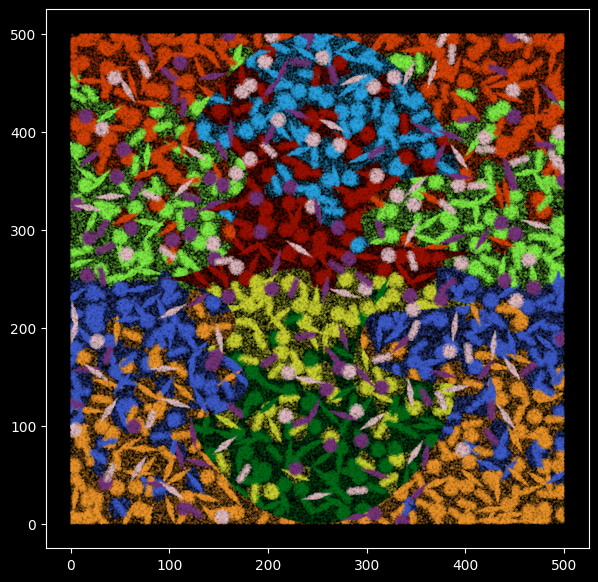
In the plot below, each data point represents one RNA transcript and has been colored by the cell type it comes from.
We simulated transcripts for a 500 by 500 square tissue for 10 cell types with different shapes and sizes.
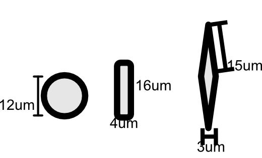
Figure 1:Sizes of simulated cell shapes.
plt.style.use('dark_background')
plt.figure(figsize=(7,7))
plt.rcParams['figure.facecolor'] = 'black'
plt.scatter(y = ground_truth_label.X,x = ground_truth_label.Y,s=0.01,
            c=[c_array[color_m[x]] for x in ground_truth_label.cell_label],alpha=0.8)
Apply GNN to learn spatial neighbourhoods of molecules in the tissue
Building RNA-transcript spatial graphs
We next construct a spatial graph for all the mRNA transcripts in the simulated dataset. In this graph, each node represents a transcript, we connect nodes when their physical distance is smaller than a radius_r, i.e., edges are added between transcripts that sit close (< radius_r)in the physical space. We initialize each node’s input feature with the transcript’s gene labels after one-hot-encoding transformation. The graph is stored as torch_geometric.data.Data.
Format directory to use SpatialRNA on the simulated data
We will use the SpatialRNA function for constructing the graph data from the input transcripts. SpatialRNA expects input files in a certain directory structure, for example, for sample_x,
./data_dir/sample_x/raw/sample_x.csv,where sample_x.csv is the CSV file with list of detected transcripts (aftering removing non-gene transcripts, i.e., control probes).
!mkdir -p '../data/sim_sample/raw/'
!zcat ../data/matrix.tsv.gz | tr '\t' ',' > ../data/sim_sample/raw/sim_sample.csv
Filtering of low-quality and control scripts
An important step of preparing the input transcripts is filtering of low-quality and control scripts. For this simple simulation data, there is no NegControl probes in the list of detected transcripts, however in real data analysis filtering of negative control step is required.
Now we can move to the application of spatialRNA in next tutorial 02